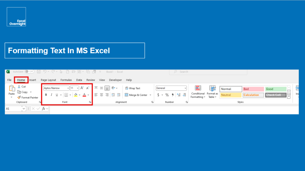
Formatting Text In MS Excel

 

Introduction

Like in any other software where you work with text, numbers, and data, you will need to format them.

Sometimes, there are company regulations like specific brand colors, specific font styles, or specific font sizes. Or perhaps, you work in academics, where the rules for formatting scientific texts or thesis are even more strict.

So, even if the right format of an Excel workbook or worksheet is trivial, it is not unimportant.

In this article, we will check some basics of formatting text in MS Excel, some advanced formatting stuff, and how to do conditional text formatting as well.

Furthermore, we will discover some formulas you can use to format text. These are called text functions.

 

Why Format Text in Excel?

Besides the regulations of your company or university, a proper text format in Excel makes perfect sense for enhancing readability and presentation. Plus, when you highlight important information in your files it helps to organize your data efficiently.

 

Basic Text Formatting

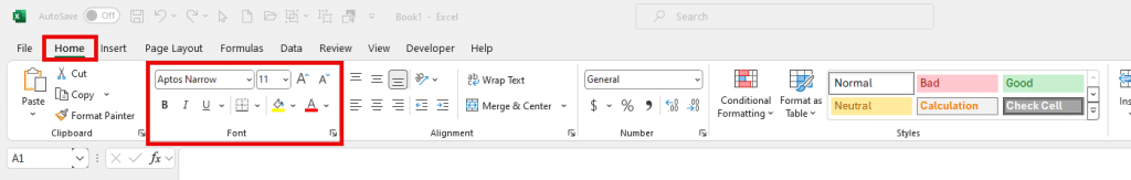
The features for text formatting in MS Excel are in the Font Group. You can find it in the Home Tab of the MS Excel Ribbon.

Font Styles and Sizes

In the Font Group (image above) there is a text field and a numbers field. These are currently showing “Aptos Narrow” and “11”. You can change the Font Name (= Font Style) into another Font by clicking the arrow of the dropdown list. Alternatively, you can start to type in the text field and overwrite “Aptos Narrow” with another Font name. The dropdown list will then pop up and guide you to the font you typed in. The same goes for the font size. You can change the font size “11” to another font size by clicking on the arrow for the dropdown list or by putting the font size you want into the numbers field manually.

Font Color

For applying different colors to your text you can use the Icon with the “A” and the colored line below the A. In the picture above this color is currently red. If you want to change the text color, you can click on this icon and a color palette will open where you can select different colors for your text. In general, you should use a different text color only for highlighting. It is best practice to not overdo it with colors. The less, the better.

Bold, Italic, and Underline

Below the text field with the font style dropdown, you can find the icons for using bold, italic, and underlining. Usually, bold fonts are for emphasis, italic fonts are for distinction and underlining fonts are for highlighting key points in a text. It is important not to mix up the underlined text with hyperlinks (to websites). For hyperlinks, there is another feature in MS Excel, which will be shown in another article. As well as with font colors, it is important not to use the bold, italic, and underline features too often. You should avoid any distractions in your files and help the user to focus on the important parts of your files.

Advanced Text Formatting

Text Alignment

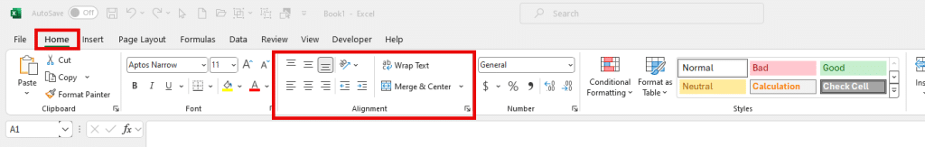
With the features in the alignment group, you can do all kinds of text alignments. The icon symbols are self-explanatory and their lines show how your text will be aligned when you click on them. Horizontal and vertical alignment are typically used very often. Indenting text can also be a feature you might want to use in some cases.

Text Wrapping

If your text is longer than your column span, but you don’t want to enhance the span horizontally, then text wrapping could be the way to go. When clicking on “Wrap Text” the text will be shown in multiple lines of the same field and the field span will be enhanced vertically. 

Merging Cells

Sometimes you need to combine and merge cells to create headers or large text blocks. In those cases, you can use the merging cells feature below the wrap text feature in the alignment group.

Conditional Formatting for Text

Applying Conditional Formatting

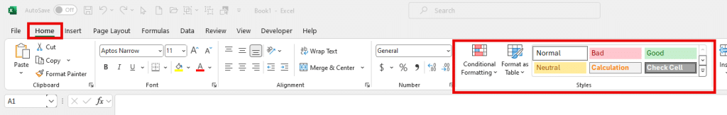
Conditional formatting is the option to change the format of your text, cells, ranges, or worksheets when pre-defined rules apply. You can find the conditional formatting feature in the left corner of the styles group in the Home Tab of your MS Excel Ribbon. Using color scales, icon sets, and data bars for specific outputs can be very handy to simplify the workbook for the user. He can then see at a glance, what the main “story” behind the data is. Especially, when you create dashboards for your data, conditional formatting is a must.

We will cover conditional formatting in a separate article, due to the complexity of the topic and the variety of the options.

Practical Examples

Highlighting duplicates and changing text color based on conditions would be practical examples of using the conditional formatting feature.

 

Working with Cell Styles

Applying Built-in Styles

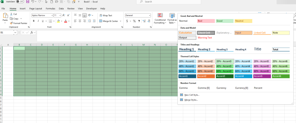
In the styles group of the MS Excel Ribbon you can select built-in styles (pre-defined). Just click on the arrows of the dropdown on the right side to open the built-in styles and select the one you like to use.

 

Creating Custom Styles

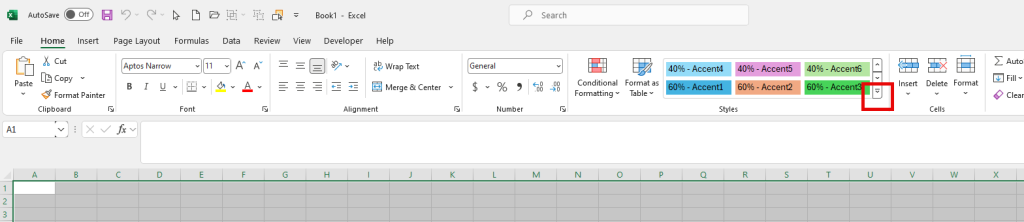
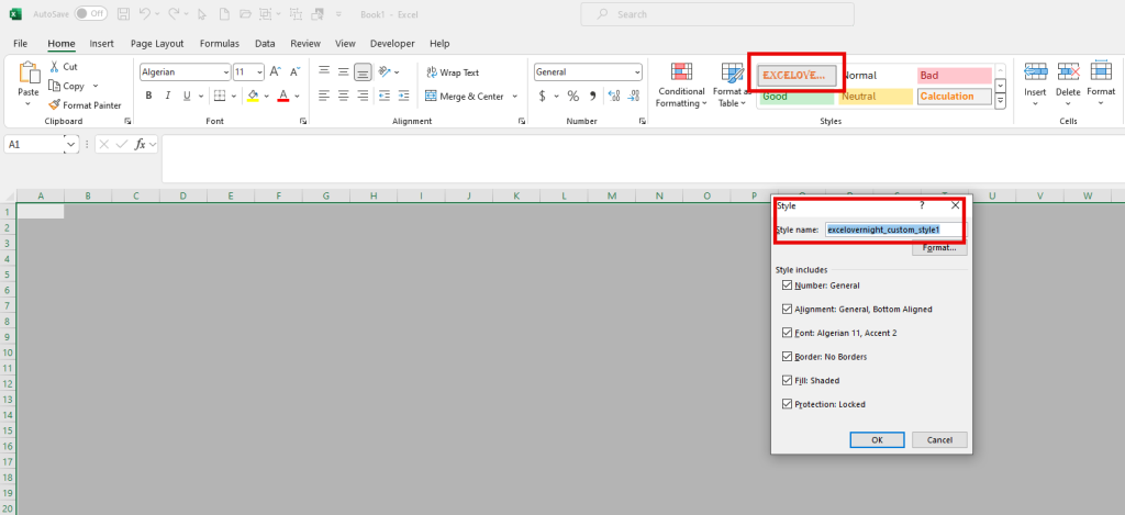
In MS Excel you have also the option to create and save custom cell styles. For this option first select the cells you want to format, then the dropdown button in the styles group…

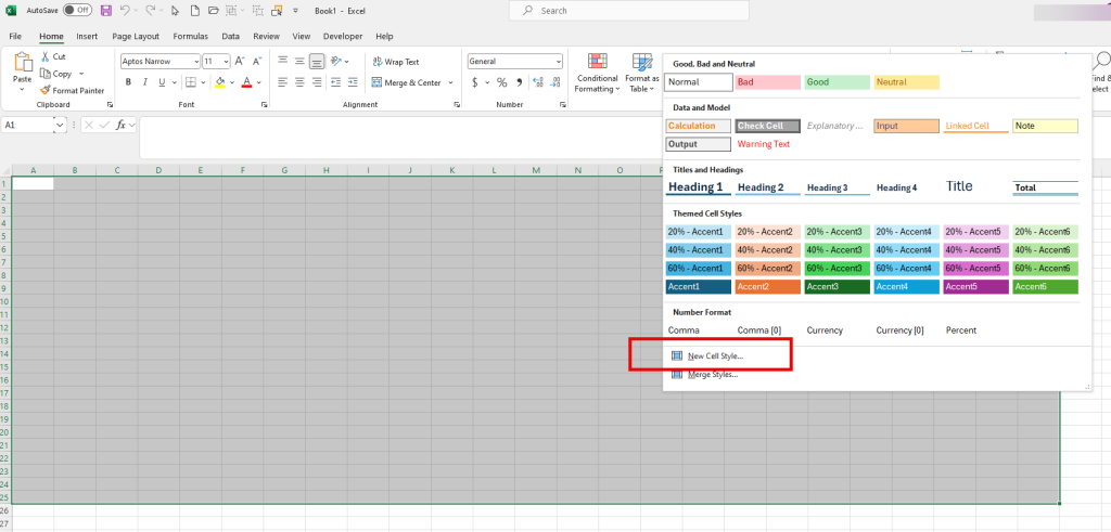
… then click on “new cell style”…

… then give your new style a name and format the style with the help of the popup window.

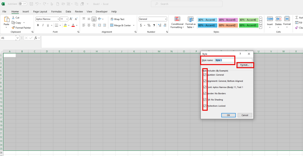
Whenever you want to use the style in the future, you can select it by the name you have given it. With a click on the right mouse button, you can modify or delete this style if you want to change it or don’t use it any longer.

Designing and saving custom styles for text are great when you use the same styles regularly. You can then simply select the pre-defined custom style and don’t need to create a new custom style with every new worksheet.

 

Using Formulas for Text Formatting

Text Functions

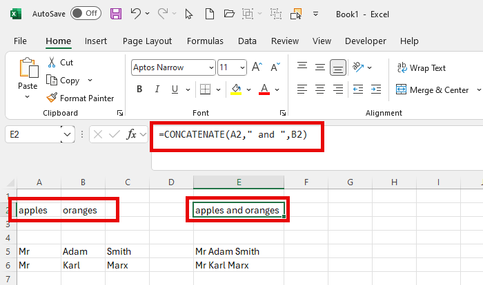
When working with the worksheet you can also use text functions like CONCATENATE or TEXTJOIN to combinate text and values and return the result as text.

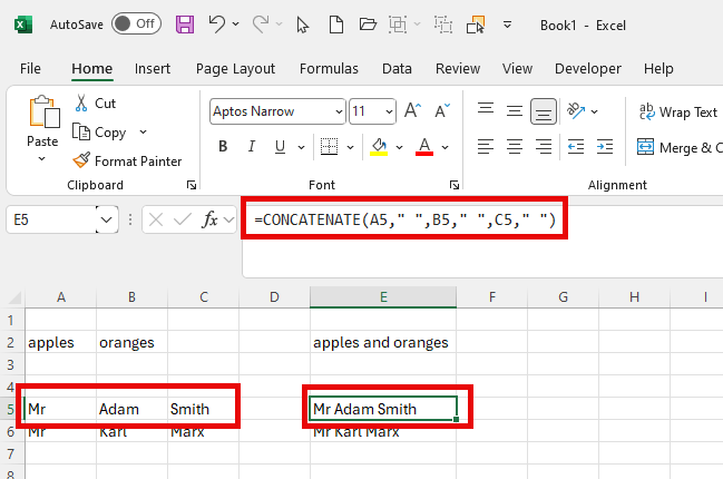
With the TEXTJOIN text function, you can combine cells as well, but spare-out empty cells. Like in the example above, the formula would be:

=TEXTJOIN(” “,TRUE,A5:D5)

The cell range would be A5 to D5 with D5 as an empty cell. With the value TRUE the TEXTJOIN function handles only cells with a value, not empty calls. So D5 will be ignored in the result in cell E5.

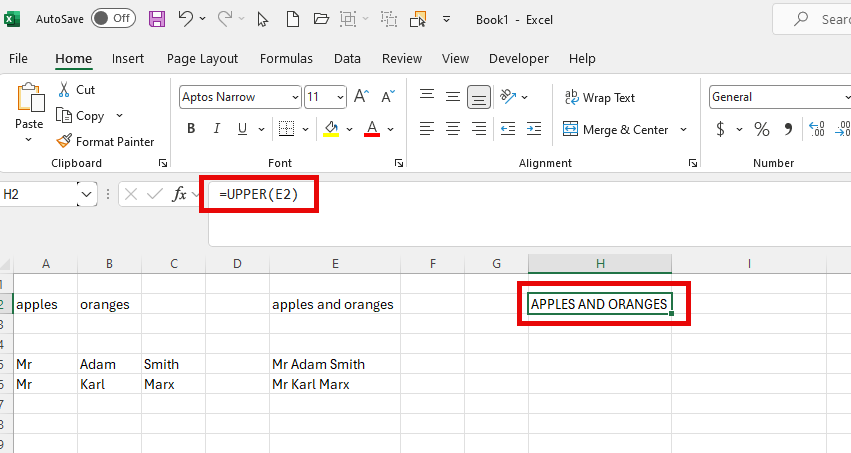
With the UPPER function, you can manipulate a text to change into upper cases, like in the example below. Cell H2 shows the value of cell E2, but in upper cases.

Conditional formatting of a cell can be done by using the IF function to apply conditional text format. We will write a separate article only for conditional formatting, due to the complexity of this topic.

 

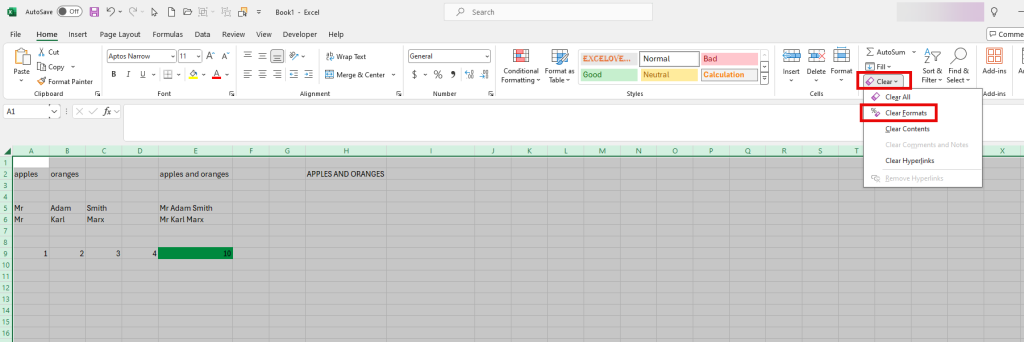
Clear Formatting

Sometimes you want to clear your old formatting and want to do a revamp of your Excel worksheet design. In this case you can select the clear format option in the MS Excel Ribbon and clear the formatting for the selected cells or worksheet.

 

Best Practices

Before formatting your text and your worksheet you should always have the user in mind. Maintaining clean and organized worksheets will help the user, to focus on the key data and key conclusions of your worksheets.

The pre-made designs of MS Excel you can find in the styles group of the ribbon work very well. Usually, for 99% of the cases, they will be enough and you don’t need to create any new text formatting beyond the existing.

If you need to format with a new style you created on your own, don’t overdo it.

Keep the same color styles throughout your workbook. Don’t change from a red color scheme to a blue color scheme with every worksheet in your workbook.

 

Conclusion

Formatting your worksheets properly can help you to present your workbooks in a professional, clear, and concise manner.

The user should get the data, the message, and the story behind the data as convenient as possible. For this reason, less is usually more.

As a workbook creator, you should always be encouraged to try new things, new formulas, and new designs.